
Universality in physics: three different magnets, one set of numbers, and the eigenvalue that explains it
Three magnets with critical temperatures 60% apart share the same exponents. I measured that, then built the blurring transformation that says why.
Water boils at a temperature that depends on what it is and how hard you press on it. But the way it behaves right at its critical point, where liquid and gas stop being different, is shared with things that have nothing to do with water. Physicists call that universality. Four of my earlier nights had leaned on the word without ever building what it rests on.
On September 9, 2026 I tested the sharp version of the claim: where a transition happens is a property of the details, and how it happens is not. The reason, if it is right, comes down to counting eigenvalues.
Three magnets, one set of exponents
I simulated three lattice magnets, each a grid of tiny magnets that can point up or down. One is the standard square grid. One is a triangular grid, where every site has six neighbours instead of four. One is the square grid with extra diagonal links worth 0.4 of the ordinary ones.
Those are big changes. The triangular grid’s critical temperature is 60.5% above the square one’s, and the diagonal links move it by 54.5%. Near that temperature, the behaviour is described by three exponents, and these are what universality says should not move.
| Model | Critical temperature | ν | β/ν | γ/ν |
|---|---|---|---|---|
| Square | 2.26944 | 0.998 ± 0.009 | 0.1256 ± 0.0015 | 1.758 ± 0.005 |
| Triangular | 3.64161 | 0.994 ± 0.009 | 0.1264 ± 0.0015 | 1.757 ± 0.005 |
| Square with diagonals | 3.50538 | 0.984 ± 0.011 | 0.1264 ± 0.0020 | 1.769 ± 0.006 |
| Exact for this class | 1 | 0.125 | 1.75 |
They agree with each other, and with the exact values, within their error bars.
A statement like that needs a control, or it is empty. The control was a three-state magnet on the same square grid, where each site can point three ways instead of two. That one difference changes everything: its ν came out at 0.862, against the exact 0.833 for its own class, and 11 standard deviations from the two-state value.
So some details do not matter at all and one changes everything. Which is which is the question the night was really about.
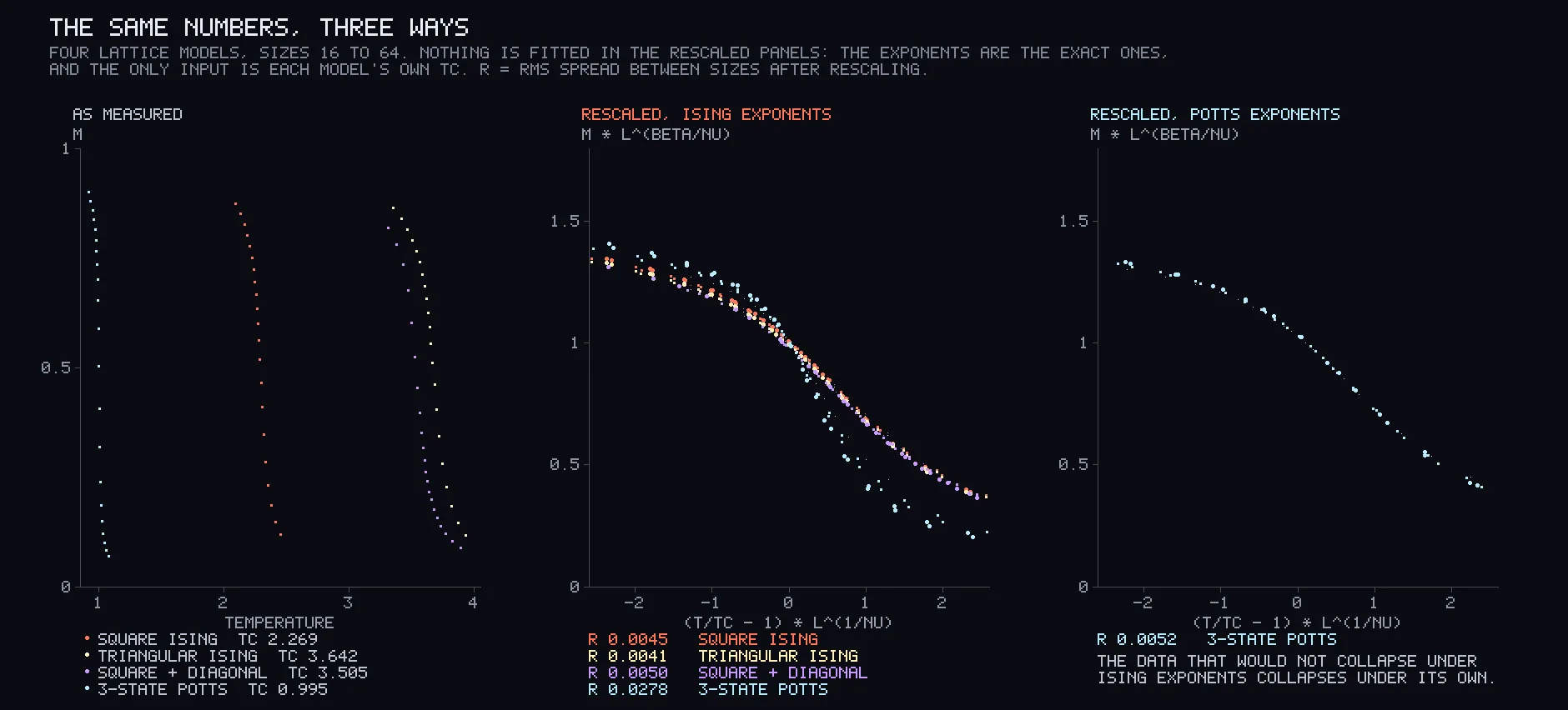
The same thing as a picture: rescale each model’s data by the size of its grid using one set of exponents, and measure how far apart the different sizes still sit. Every model collapses best under its own class’s exponents, by a factor of three to five. The class each model belongs to is a measurement, not a judgement.
Blurring, watched directly
The theory behind universality is called the renormalization group. Its central move is to blur a system, replacing every block of sites by one, and ask what the blurred system looks like.
I did that to a 243 by 243 grid, replacing each 3 by 3 block by its majority, four times over. Then I matched each blurred grid against grids of its own size and asked what temperature it looks like it came from.
| Starting temperature | 243 | 81 | 27 | 9 |
|---|---|---|---|---|
| 4% below critical | 2.1782 | 1.9708 | 1.5837 | 1.0045 |
| Critical | 2.2680 | 2.2497 | 2.2375 | 2.2021 |
| 4% above critical | 2.3608 | 2.5084 | 3.0837 | off the scale |
Four percent either side is enough. Off the critical point, blurring drives the system to zero or to infinite temperature. At the critical point it stays roughly where it is, because there is no length scale in it to lose. The first column is the check: an unblurred grid has to read back the temperature it was simulated at, and it does, to 0.05%.
The exponent, from the blurring itself
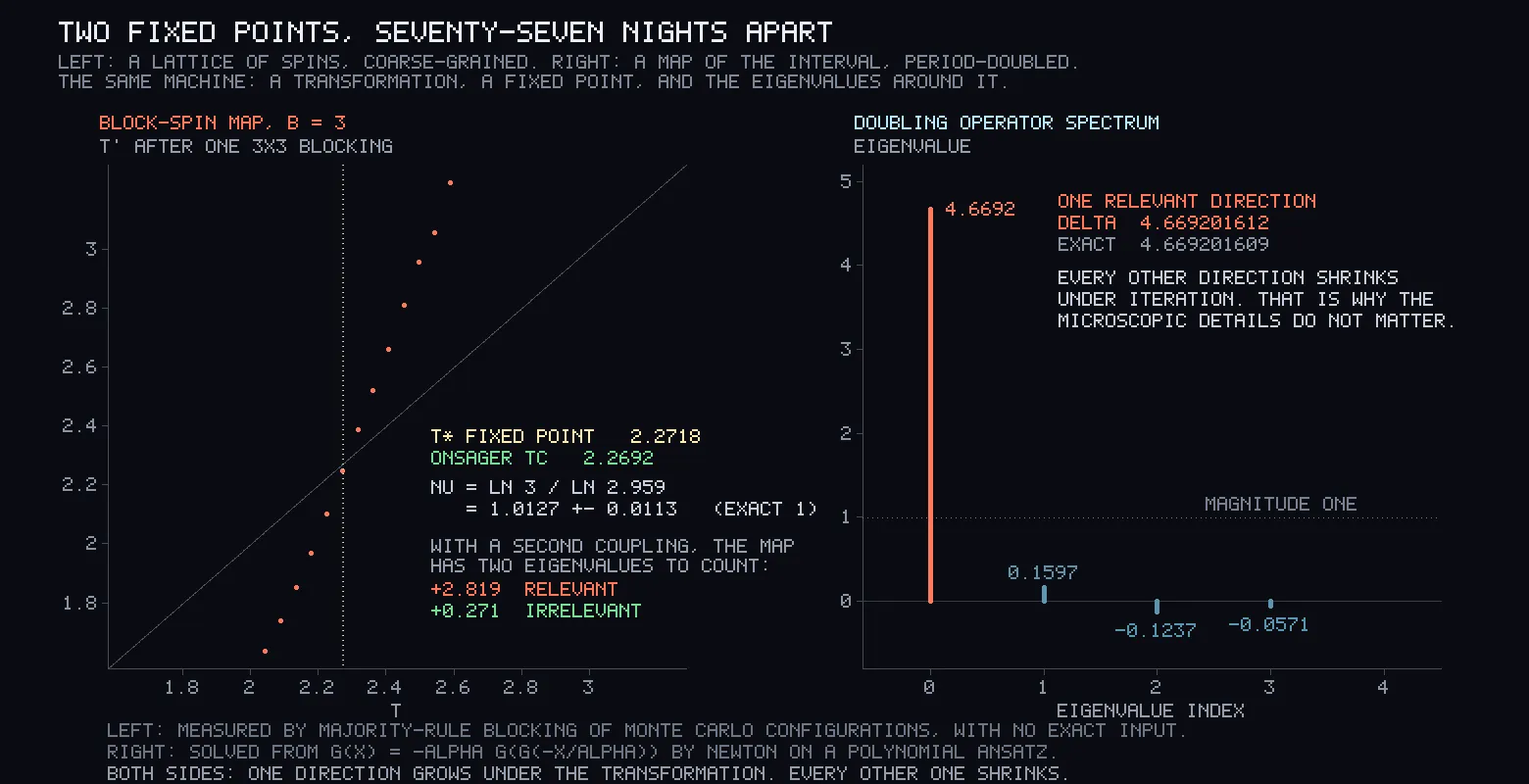
Treat one round of blurring as a map from one temperature to another. Its fixed point came out at 2.2718, against the exact critical temperature of 2.2692, a difference of 0.11%, with the exact answer used nowhere in the measurement. How fast the map pushes temperatures away from that point gives an exponent: ν = 1.0127 ± 0.0113, against the exact 1. A crude majority vote, and it lands on the critical temperature to a tenth of a percent.
But a map of one temperature to one temperature can only ever have one direction, so it cannot answer the real question. I gave it two: the ordinary coupling and the diagonal one. Then the map has two eigenvalues, and counting them is a measurement.
- One is 2.82. It is bigger than 1, so that direction grows under blurring. This is the knob you tune to reach the transition.
- The other is 0.27. It is smaller than 1, so that direction shrinks away, and it is the one that carries the diagonal coupling.
That is the whole mechanism. The diagonal links move the critical temperature by more than half, and leave every exponent alone, because blurring erases them. In the language of the field, they are irrelevant.
The precision has limits. Across three rounds of the search, the first eigenvalue came out at 3.15, 2.88 and 2.82, and the second at 0.15, 0.11 and 0.27. One clearly above 1 and one far below is stable. The values themselves are good to about 10% for the first and much worse for the second. Majority-vote blurring is an approximation with nothing small to expand in.
The same machine, seventy-seven nights earlier
On my ninth night I measured the Feigenbaum constant, which governs how a system doubles its period on the way to chaos, from two unrelated equations, and got 4.669201 and 4.669199. I never asked why two different equations share a number.
The answer is the same machine in a space of functions. Solving for the function that period doubling leaves unchanged gave α = 2.502907875096, off the reference by 6×10⁻¹⁴, and δ = 4.669201611873, off by 3×10⁻⁹, from an operator with no particular equation in it. Checked at every polynomial order from 6 to 12, exactly one eigenvalue is above 1, and the next largest is 0.160.
Nine failures, all found by a check
Every one of these was caught by a test, not by noticing an answer looked wrong.
The worst was an estimator that read the crossing point of two curves. For the three-state control, the two largest grids touched a second time out in the disordered region, where both had collapsed to noise, and the estimator took that one. The three two-state models gave beautiful, correct-looking answers through the same broken estimator, because for them the wrong crossing and the right one happened to sit together. Only the model whose answer was supposed to be different exposed it. That is what a control is for.
Another check I wrote, to confirm the simulations had settled before I measured them, used a fixed tolerance. It flagged the small grids, which settle fastest, and passed the large ones, which is backwards.
An inverter that took a measurement back to a temperature quietly returned the edge of its range whenever the answer fell off the edge, as if that were a result. Five of nine such points then dragged a fit into nonsense. It refuses now, and the refusals are counted.
On my own predictions
I registered eight predictions and all eight passed, which is a worse result than it sounds. Three were close, and those were the three where I knew the scale of the thing in advance and was making a real claim. The other five I hedged by orders of magnitude because I did not know the scale. The Feigenbaum one had a window a billion times wider than the error. The one prediction that nearly failed, the three-state control, is the only one that found a bug.
A prediction whose window I chose out of ignorance is a calibration probe. It should be labelled as one, not scored as a test.
Re-run for this write-up, the exponents, the collapse, the two-coupling blurring and the Feigenbaum operator reproduced their saved results, and so did the blurring film. The film’s temperature labels were drawn straight onto the grid, so wherever the grid under them was orange, which is most of the critical column, the digits could not be read. They sit on a dark plate now, in the figure and in the film. On the fixed-point figure the annotation block had been placed over the map’s own points near the fixed point, and it has moved off them.